Recursion: In Computer Science

Image Source: Recursion: The Pros and Cons
Original creator unknown
Definition
Recursion (noun): See recursion.
Introduction
When I was in elementary school, I lived in a dormitory with my classmates, and we all had daily chores. These chores ranged from sweeping to mopping and other tasks to keep our hostels and school tidy. Back then, I wasn’t exactly a fan of cleaning. I saw beauty in disorder and only did my duties to avoid trouble. However, one item always captivated me: the RoyalMop bucket.
At first glance, it was just an ordinary blue mop bucket, like any other. But what fascinated me was the label on the side. The label showed a picture of the mop bucket—including the label itself. This meant the image on the label contained another image of the mop bucket, which in turn had another label, and so on. In theory, this created an infinite loop of mop bucket images, spiraling deeper and deeper into itself.
I was mesmerized by this design. The bucket’s label was like a window into an endless series of smaller and smaller buckets, each one a reflection of the larger one. It was a simple object, yet it held an infinite pattern within it—so each time I saw it, I couldn’t help but pause and stare.
Years later, I found myself thinking about that mop bucket when learning about recursion in computer science. Like the label on that bucket, recursion involves a process that repeats within itself, potentially ad infinitum. It’s the same concept: something self-referential, infinitely repeatable. While searching for resources while writing this blog post, I stumbled upon images of the same RoyalMop bucket that had fascinated me years ago. The quality of the image may not be high-definition, but the recursive design still shines through.
Take a look for yourself. Notice how the label depicts the bucket, and within that, another label, and so on. It’s a real-world example of what happens under the hood of recursive implementations in computer science.


Image Source: Celplas Mopping Bucket
Recursion in Computer Science
Now, let’s jump from my elementary school days to the world of integrated circuits, machine code, and programming. In this context, recursion is a programming technique where a function calls itself to solve smaller instances of the same problem.
A recursive approach works by breaking a larger problem into smaller, more manageable pieces, each of which is a simpler version of the original task. For example, imagine you have a function that can print a single character, and your task is to print the phrase hello world. You can break this problem into smaller chunks: h, e, l, and so on. The function can then handle each character one by one until the entire phrase is printed.
This way, recursion simplifies complex tasks by tackling them piece by piece—just as that infinite series of mop bucket images breaks down into smaller and smaller reflections of itself.
In Python, this concept could be implemented using a function print_one_character to print a single character:
def print_one_character(char):
    # This function prints a single character
    print(char, end="")
We can then use this function in a recursive function, print_string_recursively, which continues calling print_one_character until all the characters in the phrase are printed:
def print_string_recursively(string):
    # If the string is empty, stop the recursion (we are done printing)
    if len(string) == 0:
        return
    else:
        # Call `print_one_character` to print the first character of the string
        print_one_character(string[0])

        # Recursively call `print_string_recursively` on the remaining part of the string
        # For example, after printing `h`, the function is called on 'ello world' for `e` to be printed next and so on
        print_string_recursively(string[1:])
Using this simple premise of breaking a problem down into smaller, similar subproblems, recursion becomes an invaluable tool, especially in problems like searching through file directories, sorting data with algorithms like merge sort, or working with hierarchical structures like trees. Its ability to handle self-similar, nested tasks with elegance and simplicity makes it indispensable in many fields of computer science, from data processing to AI algorithms.
Key Components of Recursion
A recursive implementation relies on two critical components: the base case and the corresponding recursive case. The base case is crucial because, while recursion allows a function to repeat indefinitely, we typically want it to stop once the problem is solved. The base case defines the condition under which the recursive function stops calling itself, preventing infinite recursion. Without a base case, the function would continue to call itself indefinitely, eventually causing a stack overflow (we’ll dive into that later 😉).
Here’s an example using a factorial function:
def factorial(n):
    if n == 0:  # Base case
        return 1
    else:
        return n * factorial(n - 1)  # Recursive case
In this example, the base case occurs when n == 0. At this point, recursion stops, and the function returns 1. Every recursive function needs at least one base case to ensure the recursion eventually halts.
On the other hand, the recursive case is where the function calls itself with a modified input—typically a smaller or simpler version of the original problem. In the factorial example, the recursive case is n * factorial(n - 1). Each time the function calls itself, it reduces the problem by decrementing n by 1, gradually moving toward the base case. This recursive structure breaks the problem into smaller parts, eventually converging on the base case.
The interaction between the base case and the recursive case ensures that recursion solves progressively smaller subproblems and then combines the results when the base case is reached. For example, if we calculate factorial(4), the execution would look like this:
factorial(4): return 4 * factorial(3)
    factorial(3): return 3 * factorial(2)
        factorial(2): return 2 * factorial(1)
            factorial(1): return 1 * factorial(0)
Here, our base case, factorial(0) ", yields 1. Once we hit this final result, we combine it with the previous results. factorial(1) computes 1 * 1 = 1, which we then use to compute factorial(2) as 2 * 1 = 2. Next, we compute factorial(3) as 3 * 2 = 6, and finally, we compute factorial(4) as 4 * 6 = 24`, giving us the final combined result.
Another Example: Fibonacci Sequence
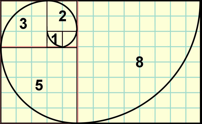

Image Sources: Fibonacci Numbers, Exploring the Fascinating World of the Fibonacci Sequence
Here’s another example of a recursive implementation: the Fibonacci sequence, which is a common use case of recursion in programming.
The Fibonacci sequence is a series of numbers where each number is the sum of the two preceding ones. The sequence typically starts as: 0, 1, 1, 2, 3, 5, 8, 13...
The Fibonacci sequence can be defined recursively, because each Fibonacci number is the sum of the two preceding numbers, except the first two numbers in the sequence: fibonacci(0) = 0 and fibonacci(1) = 1. These two serve as our base cases. Here’s the function definition below:
# recursive fibonacci function
def fibonacci(n):
    if n == 0:  # Base case 1
        return 0
    elif n == 1:  # Base case 2
        return 1
    else:
        return fibonacci(n - 1) + fibonacci(n - 2)  # Recursive case
Now, let’s evaluate the cases:
-
Base Cases:
- The base cases stop the recursion from going on indefinitely. We know that the first two numbers in the Fibonacci sequence are predefined as
fibonacci(0) = 0andfibonacci(1) = 1. - When
nreaches either0or1, the function will return0or1respectively, stopping further recursion for that branch. - We could also simplify the base case by returning
nwhenn == 0 or n == 1orn < 2. However, in this example, we explicitly define two base cases for clarity.
- The base cases stop the recursion from going on indefinitely. We know that the first two numbers in the Fibonacci sequence are predefined as
-
Recursive Case
- The recursive case is where the function calls itself. For all
n > 1, the function calls itself twice:fibonacci(n - 1)andfibonacci(n - 2), summing these two calls to get the `n’th Fibonacci number. - This recursive structure reflects how the Fibonacci sequence is built, as each number in the sequence is the sum of the previous two numbers.
- The recursive case is where the function calls itself. For all
Let’s break down the execution:
What if we want to compute fibonacci(3):
-
Intiail call:
fibonacci(3)- Since
nis not0or1, we enter the recursive case:fibonacci(3) = fibonacci(2) + fibonacci(1).
- Since
-
Evaluate
fibonacci(2):- Similarly,
fibonacci(2)triggers the recursive case:fibonacci(2) = fibonacci(1) + fibonacci(0).`
- Similarly,
-
Base cases
fibonacci(1)andfibonacci(0)`:fibonacci(1)hits the base case and returns1.fibonacci(0)also hits the base case and returns0.
-
Unwinding the recursion:
-
Now, we combine the results, starting from the base cases:
fibonacci(2) = 1 + 0 = 1.- And finally,
fibonacci(3) = fibonacci(2) + fibonacci(1) = 1 + 1 = 2.
-
The final result of fibonacci(5) is 5.
Real-world Applications of Recursion
Recursion has various real-world applications across multiple domains, from sorting algorithms to tree data structure and dynamic programming. I’ll discuss some of these applications in detail below:
Divide and Conquer Algorithms
Divide and conquer algorithms are almost inherently recursive, as the logic is to “divide” a problem into smaller subproblems, which are easier to solve, and then “conquer” each subproblem recursively before combining the results to get the final solution. Two popular examples of divide and conquer algorithms are merge sort and quick sort:
Merge Sort: This algorithm divides an unsorted list into two halves, recursively sorts each half, and then merges the sorted halves. For example, if we need to sort a list of numbers, merge sort recursively splits the list in half until it reaches sublists of size 1, which are inherently sorted, and then merges them. Below is a good graphic on how this algorithm proceeds:
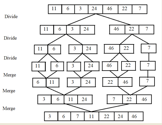
Image Source: Understanding Merge Sort Algorithm with Java Source Code
Quick Sort: This algorithm works by selecting a “pivot” element from a list of items, partitioning the remaining elements into two sublists based on whether they are less than or greater than the pivot, and then recursively applying the same process to the sublists. Once the base case (an empty or single-element list) is reached, the recursion unwinds, and the fully sorted list is returned. This recursive partitioning enables quicksort to handle large datasets efficiently.
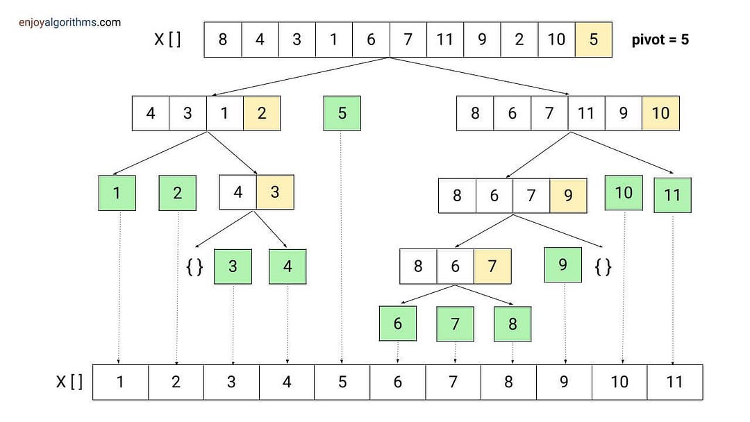
Image Source: Quick Sort Algorithm
Tree Traversals
Recursion is also a powerful tool for traversing tree structures such as binary trees, binary search trees, and decision trees. In tree traversal, each node in a tree has a similar structure, consisting of a value and links to its child nodes. Recursion is ideal for this task, as it allows the traversal function to explore nodes in a specific order. The base case will be an instance where a node has no children, while the recursive case involves calling the traversal function on the children of the node—thus moving through the tree. It is pretty elegant how tree traversals are implemented recursively. You can read more about them in these articles: 4 Types of Tree Traversal Algorithms, Navigating Trees: In-Depth Look at Traversal Algorithms.
Dynamic Programming
In dynamic programming, recursion is often combined with memoization to solve problems more efficiently by avoiding redundant computation. In cases where recursion might be inefficient due to repeated calculation of the same subproblem, dynamic programming offers an optimized approach by storing the results of expensive function calls and reusing them when needed.
A classic example of recusion and memoization is the Fibonacci sequence. In a naïve recursive implementation of the Fibonacci sequence, the function repeatedly recalculates the same Fibonacci numbers, leading to exponential time complexity. For example, to calculate fibonacci(5), the recursive function calculates fibonacci(4) and fibonacci(3), but to compute fibonacci(4), it again calculates fibonacci(3), creating a lot of redundant work.
To optimize this, memoization stores the result of each Fibonacci number once it’s computed, so the function doesn’t have to recompute it in future calls. Here’s an optimized version using recursion and memoization:
def fibonacci(n, memo={}):
    if n in memo:
        return memo[n]
    if n == 0 or n == 1:
        return n
    else:
        memo[n] = fibonacci(n - 1, memo) + fibonacci(n - 2, memo)
        return memo[n]
By storing the results of subproblems in the dictionary (memo), this version of the Fibonacci function ensures that each Fibonacci number is only computed once, reducing the time complexity from exponential to linear.
Recursion and memoization are frequently used in a wide range of dynamic programming problems such as knapsack problems, minimum edit distance (used in spell checkers or DNA sequence alignment), and longest common subsequence (used in version control systems). In each case, recursion breaks the problem into overlapping subproblems, and memoization ensures that these subproblems are not recomputed, greatly enhancing efficiency.
Other Application
Beyond the abovementioned ones, recursion is used in numerous other real-world applications. Some examples include backtracking algorithms (used in Sudoku, Maze solvers, etc.), data structure operations such as linked lists or trie data structures, web crawlers (used in search engines), expression evaluations (such as parsing nested parentheses and multiple operations in mathematical expressions), pathfinding algorithms, network protocols, robotics and simulations, image processing, social networks, and many more.
Common Pitfalls in Recursion
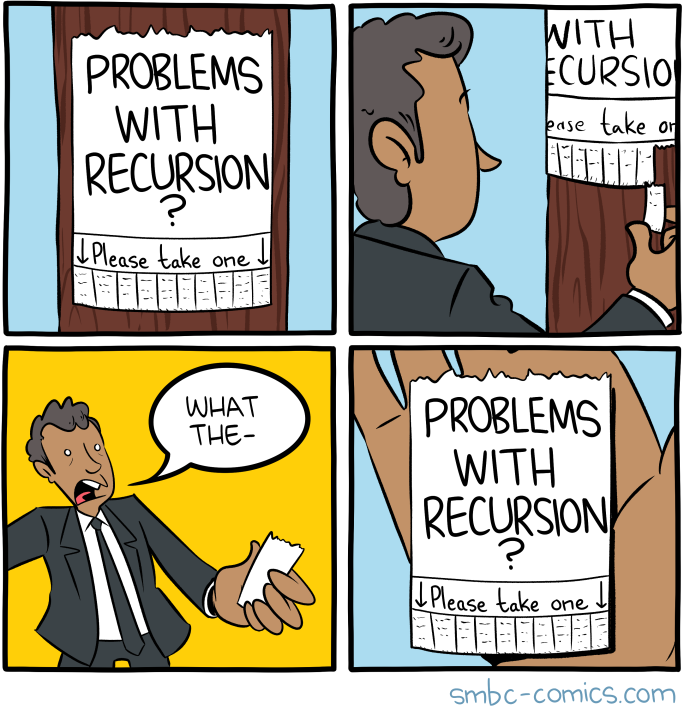
Image Source: SMBC Comics: Recursion
While recursion is a powerful tool extensively used in programming, it comes with its own set of challenges and pitfalls. The most common issues that arise with recursive algorithms are stack overflow (not the popular Q&A website for developers—even though I mischievously linked it above 😈) and efficiency drawbacks.
Stack Overflow
Before diving into stack overflow, let’s understand how the call stack works. Think of the call stack as a stack of plates in a kitchen. When you wash dishes, each time you finish cleaning a plate, you place it on top of the stack. As you keep washing more plates, you continue stacking them on top. When you’re done, you take the top plate off first, then the next, and so on—removing them in reverse order. This is exactly how the call stack works in programming: each new function call gets “stacked” on top of the previous one, and when a function completes, it is “popped” off the stack in a last-in, first-out (LIFO) manner. You can read more about the call stack in this article.
Now, imagine writing this blog post. I started by creating an outline of the concepts I wanted to cover, breaking each central idea into sections I could flesh out. I tackled each section individually, starting with the Introduction. Once I finished a section, I set it aside (popped it off my mental “stack”) and moved on to the next section. Each time I finished one section, I could remove it from my mental stack and focus on the next one.
But what if I tried to write the entire blog all at once without breaking it down? Imagine trying to tackle every section and paragraph simultaneously without giving each part my entire focus. My mind would get cluttered with all these unfinished pieces. I’d eventually get overwhelmed because my “mental stack” would become too full. This is similar to what happens in programming when too many function calls are stacked on top of each other due to deep or infinite recursion.
In the case of recursion, a new “task” is added to the call stack each time a function calls itself, just like focusing on each section of the blog. Each recursive call represents a piece of the problem the function is trying to solve. As the program finishes working on a recursive call (just like completing a section), it removes it from the stack and moves on to the previous function that called it.
If there’s no clear base case in the recursive function, or if the input size is too large, the call stack keeps growing without a way to reduce it. This is like trying to write more and more sections of the blog without finishing any of them. Eventually, I run out of focus and capacity to keep track of what I’m working on. That’s a stack overflow. Essentially, too many function calls consume memory on the system’s call stack, and the stack exceeds its limit, causing an error.
For example, consider a recursive function without a base case:
def infinite_recursion(n):
    print(n)
    return infinite_recursion(n + 1)  # No base case to stop the recursion
In the above code, the function infinite_recursion keeps calling itself indefinitely, consuming memory on the stack until the program crashes with a stack overflow error. This is why defining a clear and reachable base case is critical in any recursive function.
Even with a proper base case, deep recursion can cause a stack overflow if the input size is too large. For instance, computing large values in the Fibonacci sequence using a naïve recursive implementation can result in deep recursive calls that exhaust the stack:
def fibonacci(n):
    if n == 0 or n == 1:  # Base cases
        return n
    return fibonacci(n - 1) + fibonacci(n - 2)
For large values of n, such as fibonacci(2000), the above function will make an enormous number of recursive calls, leading to stack overflow due to the depth of recursion.
Efficiency
Another concern with recursion is its efficiency. Recursive solutions can be less efficient than iterative solutions due to the overhead of repeated function calls. Each recursive call adds an entry to the call stack, which consumes memory and takes time to set up. This overhead can significantly impact performance, especially for problems with deep or highly repetitive recursive calls.
For example, a simple loop can often achieve the same result as a recursive function with less memory usage and faster execution time. Let’s compare two implementations of factorial:
Recursive Factorial
def factorial_recursive(n):
    if n == 0:
        return 1
    return n * factorial_recursive(n - 1)
Iterative Factorial
def factorial_iterative(n):
    result = 1
    for i in range(1, n + 1):
        result *= i
    return result
The iterative approach avoids the overhead of function calls and potential stack overflow, making it more memory-efficient. However, recursion offers a cleaner, more intuitive approach in some cases, especially when working with problems with a natural recursive structure (like tree traversals).
The choice between recursion and iteration often depends on the complexity of the problem and the size of the input. For example, while recursion is elegant and simple for problems like tree traversal or divide-and-conquer algorithms, iterative solutions might be more suitable for scenarios with high memory constraints or large datasets.
These are good articles to learn more about efficiency as related to recursions: Why Recursion Is Less Efficient Than a Loop — Programming Word of the Day, Performance of recursive functions (and when not to use them)
Tail Recursion Optimization
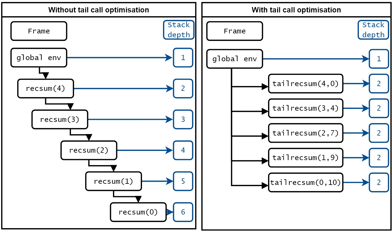
Image Source: Optimization of tail recursion in R
Tail recursion is a specific type of recursion in which the recursive call is the last operation in the function. This seemingly minor distinction is quite powerful because it enables some programming languages to optimize recursive calls to prevent stack overflow and reduce memory usage. This optimization is known as Tail Call Optimization (TCO).
What is Tail Recursion?
In a normal recursive function, each recursive call creates a new stack frame that holds information about the current function’s execution context (local variables, return address, etc.). As recursive calls accumulate, each call leaves behind an unresolved task in the stack, leading to an ever-growing stack. This is why, in deep recursion, you often encounter stack overflow errors—the call stack grows beyond its limit.
However, in a tail-recursive function, the recursive call is the very last operation that the function performs. When a recursive call is the last thing a function does, there’s no need to keep the current stack frame. This allows the language or compiler to reuse the same stack frame for the next call, essentially transforming the recursion into an iteration under the hood.
Example: Tail Recursion vs. Normal Recursion
Let’s compare a simple recursive function to its tail-recursive version. Consider a function that calculates the sum of the first n numbers.
def sum_normal(n):
    if n == 0:  # Base case
        return 0
    return n + sum_normal(n - 1)  # Not a tail call because of the addition after the call
In this example, after the recursive call sum_normal(n - 1) "is made, the function still needs to add n to the result. This creates a chain of unresolved additions that each need their own stack frame. For large values of n`, this chain can quickly lead to a stack overflow.
Now, let’s rewrite this function using tail recursion.
def sum_tail_recursive(n, accumulator=0):
    if n == 0:  # Base case
        return accumulator
    else:
        return sum_tail_recursive(n - 1, accumulator + n)  # Tail call
In this version, the recursive call sum_tail_recursive is the very last thing that happens in the function. All the necessary work (adding n to the accumulator) is done before the recursive call. There’s no further computation needed once the recursive call returns. This is the hallmark of a tail-recursive function.
How Tail Call Optimization Works
In a tail-recursive function, once the final recursive call is made, the current stack frame is no longer used. In languages that support Tail Call Optimization (TCO), the compiler can recognize that it doesn’t need to keep the current stack frame around. Instead, it can reuse the current stack frame for the next recursive call, effectively converting the recursion into an iterative process without needing additional memory.
Since TCO allows the compiler to reuse the current stack frame instead of creating a new one for each recursive call, the call stack size doesn’t grow with each recursive call. This prevents stack overflow, even if the function makes many recursive calls.
For example, in a language with TCO support (like Scheme, Haskell, Scala, and Clojure), a tail-recursive function like the one above will consume a constant amount of stack space, regardless of the depth of recursion. O, even if a function is written in a tail-recursive form, it won’t receive the same stack-saving optimizations as in other languages.
Visualizing Tail Recursion vs. Normal Recursion
Imagine you’re trying to count the number of steps on a staircase:
-
Normal Recursion: With a non-tail-recursive approach, every time you take a step, you leave a “marker” behind so you can retrace your steps on the way back. For instance, if you walk up 100 steps, you’ll leave 100 markers. When you reach the top, you have to return to each step to pick up your markers in reverse order. This is similar to normal recursion—every recursive call leaves behind some unfinished work (an unresolved operation) that needs to be revisited later. This ongoing “memory” of unfinished tasks builds up in the call stack, leading to potential stack overflow.
-
Tail Recursion: Now imagine a different approach where you don’t leave any markers behind. Instead, at each step, you update a running count and move to the next step without needing to remember where you’ve been. When you reach the top, you already have the final count—there’s no need to retrace your steps. This is how tail recursion works: each recursive call performs its work completely before moving on without leaving unresolved operations behind on the stack. This efficiency prevents the stack from growing, allowing you to handle large recursions without running out of memory.
Conclusion
I hope you enjoyed reading this blog post and learned something new. For the closing, let’s play a little game that might keep you staring at this page forever. Have fun 😅
def conclusion():
    print("Recursion is great for breaking down problems into smaller parts. But if you forget a base case, you might be stuck here forever…")
    conclusion()  # Oops, we did it!
References
While I have cited a handful of sources in this blog post, below are some other resources that I used to write it and that can be useful for your further learning.
- Project Python: Recursion
- Recursion: The Pros and Cons
- How to Think Recursively | Solving Recursion Problems in 4 Steps
- Fibonacci Numbers
- Merge Sort – Data Structure and Algorithms Tutorials
- Memoization
- What is Backtracking Algorithm? Types, Examples & its Application
- Tail Call Optimization: What it is? and Why it Matters?
- Tail-recursive algorithms
- Tail Call Optimisation in C
- What is Tail Recursion
- This is a Better Way to Understand Recursion
- 5 Simple Steps for Solving Any Recursive Problem
- Recursion
- Reading 10: Recursion
- Recursion in Python: An Introduction
- Recursion
- Recursion and Looping
- Recursion vs. Looping in Python
- Different Techniques for Iterating over Data
- Difference between Recursion and Iteration
- Benchmark: Recursion vs Iteration
- A cheap trick to speed up recursion in C++
- Optimizing Recursive Algorithms: Techniques to Reduce Space Complexity